Learning to Estimate Continuous Outcomes

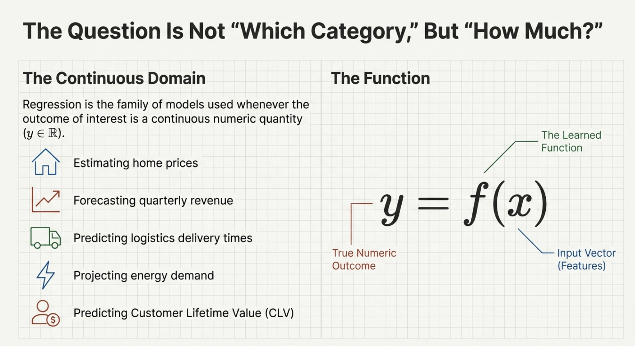
Regression is one of the most foundational problem types in machine learning. It is the family of models used whenever the outcome we care about is a continuous numeric quantity. Regression models power many of the most common predictive systems in business:

• estimating the price of a home
• forecasting revenue next quarter
• predicting delivery time for logistics
• estimating insurance claim severity
• predicting customer lifetime value
• projecting energy demand in the next hour

In all of these cases, the question is not which category something belongs to, but rather:

What numeric value should we expect?

This is the defining characteristic of regression.

3.2.1.1 Regression as Function Learning

Recall the basic structure of machine learning:

y^=f(x) Where:

• x is a vector of input features
• y is the true numeric outcome
• y^ is the model’s prediction
• f(⋅) is the learned function

In regression, the output belongs to the continuous domain: y∈R

The goal is to learn a function that produces predictions as close as possible to reality.

Example: House Price Prediction

Suppose we want to predict the sale price of a home.

Inputs might include:

• square footage
• number of bedrooms
• neighborhood
• proximity to transit
• year built
• renovation history

Output:

• sale price in dollars

The model learns:

Price = f(Size,Bedrooms,Location,Age,… )

Once trained, the model can estimate the price of new homes before they sell.

3.2.1.2 How Regression Models Learn: The Loss Function

Regression models learn by minimizing prediction error.

The most common objective is the Mean Squared Error. We discussed this WDIS AI-ML Series: Module 2 Lesson 1: Objective function - AI is nothing but an optimization problem:

This objective captures a simple principle:

A good regression model is one that makes predictions close to the true numeric outcomes.

Different regression models differ primarily in how they represent the function f(x).

3.2.1.a Linear Regression — The Starting Point

Linear regression is the simplest regression model and remains one of the most widely used tools in applied analytics.

It assumes the relationship between features and outcome can be approximated by a linear combination:

Where:

• wi are coefficients learned from data
• b is the intercept

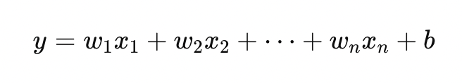
Intuition: Linear Models as Weighted Evidence

A linear regression model treats each feature as contributing additively to the final prediction.

For example:

• more square footage increases price
• better neighborhood increases price
• more bedrooms increases price

Each coefficient represents the marginal effect of that feature.

Practical Example

A trained model might learn:

Price = 200⋅Size + 15,000⋅Bedrooms+ 50,000⋅NeighborhoodScore

Interpretation:

• Each additional square foot adds $200
• Each bedroom adds $15,000
• Neighborhood quality strongly drives value

This interpretability is why linear regression is often preferred in regulated or stakeholder-heavy environments.

When Linear Regression Works Well

Linear regression performs well when:

• relationships are approximately linear
• features are meaningful and not overly complex
• interpretability is critical
• the dataset is moderate in size

It is widely used in:

• pricing analytics
• financial forecasting
• marketing mix modeling
• early-stage baselines

Where Linear Regression Breaks Down

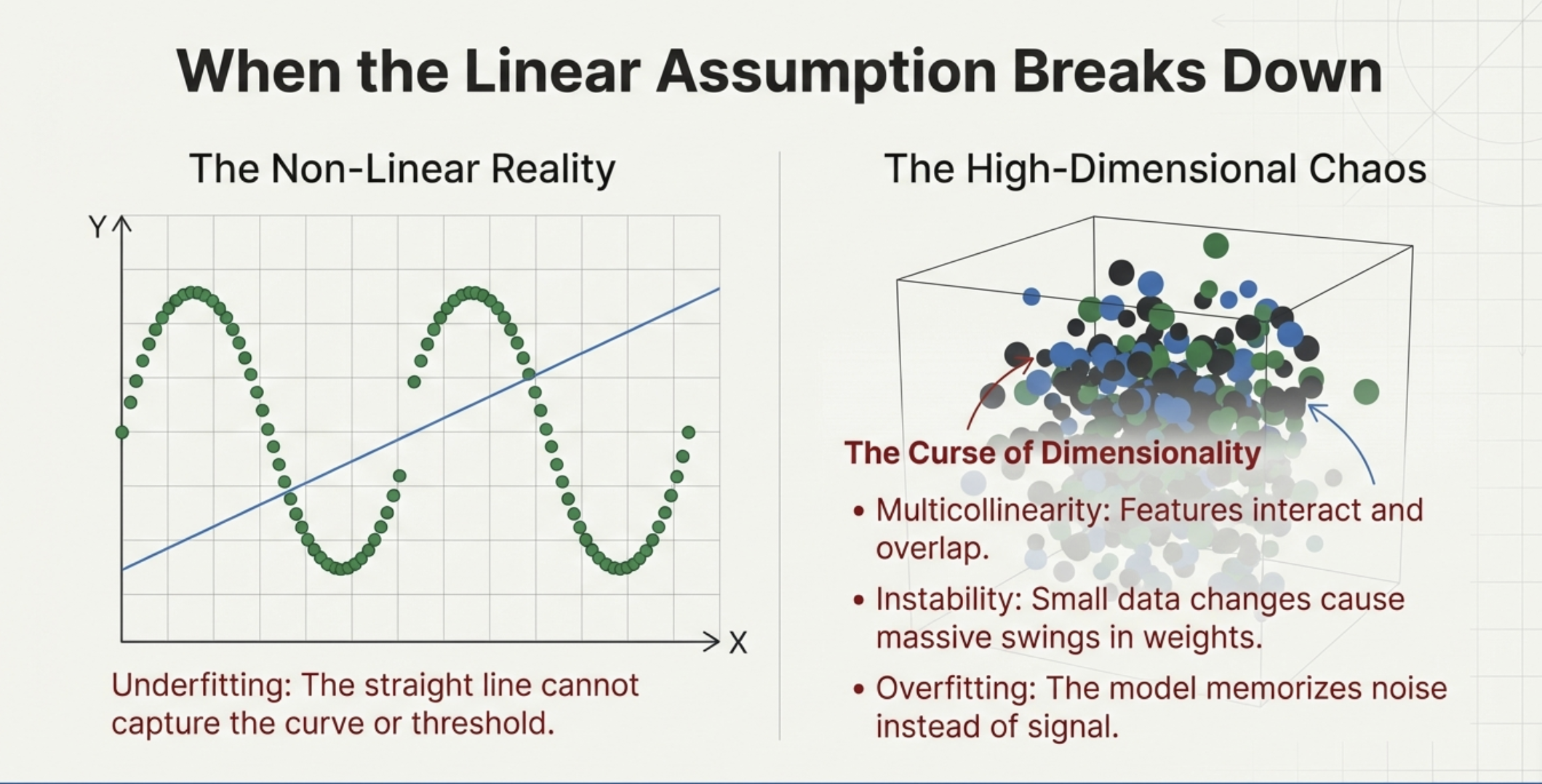
Linear regression struggles when:

• relationships are nonlinear
• features interact strongly
• the dataset contains many correlated predictors
• the signal-to-noise ratio is low

Example:

House prices do not rise smoothly. They jump sharply when crossing neighborhood boundaries.

Linear regression cannot naturally represent such discontinuities.

This motivates regularization and nonlinear models.

‍

3.2.1.b Regularized Regression

Ridge, Lasso, and Elastic Net

Modern regression problems often involve high-dimensional feature spaces. For example, predicting customer lifetime value might include:

• hundreds of behavioral signals
• marketing touchpoints
• device metadata
• product usage metrics

In such settings, ordinary linear regression tends to overfit. Why? More variables ⇒ More dimension ⇒ More chances of overfitting. We will discuss this in detail when we get to overfitting section.

Regularization solves this by penalizing complexity. So, in short it leans towards a simpler model. How? Let us look at some of the regularization techniques.

Ridge Regression (L2 Regularization)

Ridge regression modifies the loss function:

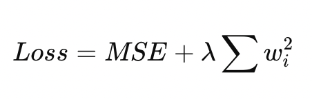
The penalty discourages large coefficients.

Why Ridge Helps

When features are correlated (common in business data), linear regression becomes unstable:

• small changes in data produce large coefficient swings

Ridge smooths the model and improves generalization.

Practical Use Case

Forecasting revenue using many correlated predictors:

• advertising spend
• promotions
• pricing
• competitor activity

Ridge regression stabilizes estimates.

‍

Lasso Regression (L1 Regularization)

Lasso adds a different penalty:

The key difference:

• Lasso can shrink coefficients exactly to zero

This makes Lasso a feature selection method.

Practical Use Case

A churn regression model with 500 features:

• Lasso may reduce this to the 20 most predictive signals.

This is valuable for:

• interpretability
• simpler deployment
• reducing noise

Elastic Net Regression

Elastic Net combines Stability and Feature Selection in High-Dimensional Settings by combining  Ridge and Lasso.

Most real-world datasets contain many features, many of which are correlated, noisy, or redundant.

In such environments, ordinary linear regression becomes unstable, and even Ridge or Lasso alone may not be sufficient.

Elastic Net was developed as a hybrid approach that combines the strengths of both major regularization methods:

• Ridge Regression (L2) for stability
• Lasso Regression (L1) for sparsity and feature selection

As a result, Elastic Net is often one of the most effective and widely used regression techniques in high-dimensional applied machine learning.

It is often the best practical choice in high-dimensional business regression problems.

Why Elastic Net Exists: The Limitations of Ridge and Lasso Alone

To understand Elastic Net, it helps to recall what Ridge and Lasso each do well—and where they struggle.

Ridge Regression: Stable but Not Sparse

Ridge regression adds an L2 penalty:

This discourages large coefficients and produces stable models when predictors are correlated.

However, Ridge has one limitation:

• It rarely drives coefficients exactly to zero.

So Ridge does not perform feature selection.

The model still includes all predictors, just with smaller weights.

This can reduce interpretability and make deployment harder when hundreds of features remain active.

Lasso Regression: Sparse but Unstable with Correlated Features

Lasso regression adds an L1 penalty:

Its key advantage is sparsity:

• It shrinks some coefficients exactly to zero
• It automatically selects a subset of features

But Lasso struggles when features are highly correlated.

In business datasets, this is extremely common:

• marketing channels overlap
• customer engagement metrics move together
• financial indicators are interdependent

In such cases, Lasso tends to behave unpredictably:

• it selects one feature arbitrarily
• it drops others even if they are equally meaningful
• small changes in data can change which features survive

‍

Elastic Net: The Best of Both Worlds

Elastic Net addresses these limitations by combining both penalties:

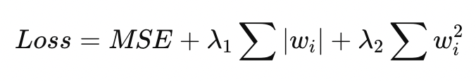
This means Elastic Net encourages:

• sparsity (like Lasso)
• stability (like Ridge)

Instead of choosing between Ridge or Lasso, Elastic Net provides a continuum between them.

Key Properties of Elastic Net

Elastic Net has three major advantages that make it especially useful in practice.

1. Feature Selection with Stability

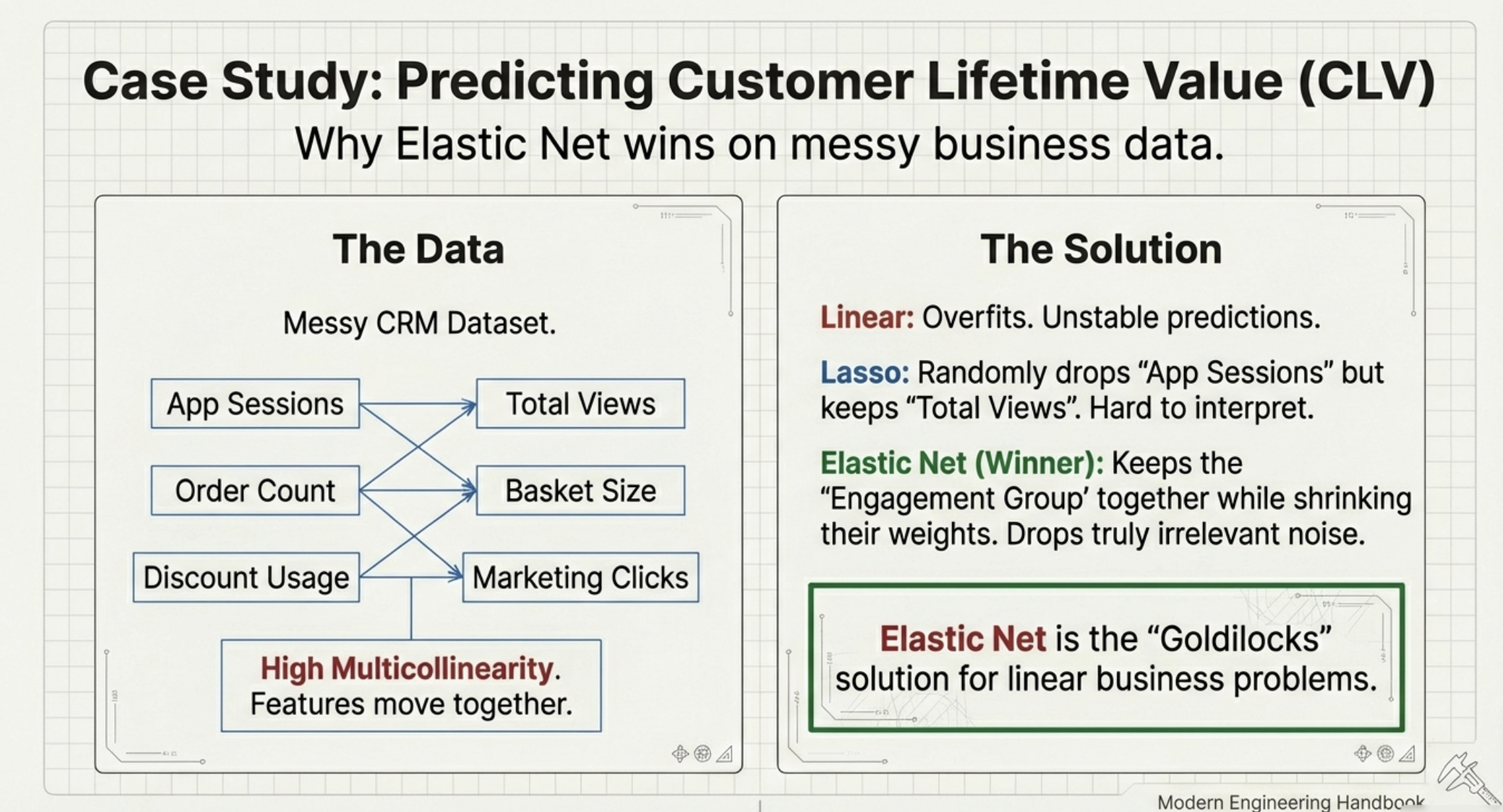
Elastic Net can eliminate irrelevant predictors, but unlike pure Lasso, it does so in a more stable way. This is particularly important when features are correlated. Instead of picking one feature and discarding the rest, Elastic Net often keeps groups of related predictors together.

Example:

• customer logins per week
• number of sessions
• time spent in app

These features are highly correlated signals of engagement. Elastic Net tends to treat them as a group rather than selecting one arbitrarily.

2. Better Performance in High-Dimensional Data

Elastic Net is especially valuable when:

• number of features is large
• many features are weak but useful
• noise is present
• multicollinearity is unavoidable

This is common in real organizational datasets:

• CRM systems
• marketing analytics
• product telemetry
• operational forecasting

3. A Practical Default for Business Regression

Because business data often has:

• many correlated predictors
• the need for interpretability
• the need for some feature selection
• the need for stability

Elastic Net becomes a highly practical “default” regression model. It often performs better than Ridge or Lasso alone in applied settings.

‍

Practical Business Example: Predicting Customer Lifetime Value

Consider an e-commerce company trying to predict:

CLV=f(CustomerBehavior, Purchases, MarketingExposure, EngagementSignals,…)

The feature set might include:

• number of orders
• average basket size
• time since last purchase
• discount usage
• email click-through rates
• app session frequency
• customer support contacts

Many of these features are correlated.

• high-value customers tend to have high engagement
• discount usage correlates with order frequency
• marketing exposure overlaps across channels

In this setting:

• Linear regression overfits
• Ridge keeps all features, reducing interpretability
• Lasso drops correlated predictors inconsistently
• Elastic Net provides both stability and sparsity

Thus, Elastic Net becomes one of the most reliable models for structured business prediction problems.

When Elastic Net is Most Appropriate

Elastic Net is particularly useful when:

• you have many features (hundreds or thousands)
• predictors are correlated
• you want feature selection but not instability
• interpretability matters
• you want a strong linear baseline before moving to trees or boosting

It is commonly applied in:

• churn value modeling
• revenue forecasting
• marketing response prediction
• credit risk scoring
• healthcare cost estimation

Elastic Net in the Regression Model Progression

In practice, Elastic Net often sits at an important point in the modeling ladder:

1. Linear Regression (simple baseline)
2. Ridge / Lasso (regularization)
3. Elastic Net (best practical linear model)
4. Tree-based models (nonlinear patterns)
5. XGBoost (industry-grade performance)

Elastic Net is often the final step in the “linear family” before organizations move to nonlinear ensembles.

Summary: Elastic Net

Elastic Net is a hybrid regularized regression model that combines:

• Ridge’s stability with correlated features
• Lasso’s ability to perform feature selection

It is one of the most practical choices for high-dimensional business regression problems because real-world organizational data is rarely clean, independent, or low-dimensional.

Elastic Net provides a balanced approach:

• interpretable
• stable
• sparse
• deployable

‍

3.2.1.c Tree-Based Regression Models

Capturing Nonlinear Relationships

Linear models assume additive relationships.

Decision trees remove this assumption.

A tree learns rules such as:

• If neighborhood = premium and size > 2000 → high price
• If neighborhood = rural and age > 50 → lower price

Trees partition the feature space into regions.

Why Trees Matter

Tree regression naturally captures:

• nonlinearities
• feature interactions
• threshold effects

Example: Square footage matters much more in expensive neighborhoods than in cheap ones. Trees represent this interaction automatically.

Strengths of Tree-Based Regression

• minimal preprocessing
• handles mixed categorical + numeric features
• interpretable as decision rules
• captures complex patterns

Weaknesses of Single Trees

Single trees are rarely deployed alone because they:

• overfit easily
• are unstable (high variance)

This leads to ensembles.

Ensemble Learning

How to combine multiple models (In this case Trees) together, In comes, Ensemble Learning

When a single model is not strong enough on its own, one of the most powerful ideas in machine learning is to combine many models together to produce a better predictor. This approach is called ensemble learning.

The central intuition is simple: a single decision tree (or model) is often unstable. It may capture patterns in the data, but small changes in the training set can lead to very different trees, and individual trees are prone to overfitting. By building multiple trees and aggregating their outputs, we can reduce these weaknesses and create a model that is more accurate, more robust, and more reliable on unseen data.

In ensemble learning, instead of relying on one tree’s judgment, we rely on the collective intelligence of many trees. Each tree acts as a “weak learner,” making imperfect predictions, but when combined, the ensemble becomes a “strong learner.” There are two primary ways to combine trees or Machine learning Models.

1. Bagging, short for bootstrap aggregating, works by training many independent models in parallel on different random samples of the training data, and then combining their predictions, typically by averaging in regression or majority voting in classification. The key intuition is variance reduction: a single decision tree is highly unstable and sensitive to small changes in the data, but an ensemble of many trees smooths out these fluctuations. Random Forest is the most widely used bagging-based method, and its strength comes from building a diverse “forest” of trees that collectively produce more robust and generalizable predictions than any individual tree.
2. Boosting, in contrast, is a sequential strategy in which models are trained one after another, with each new model focusing specifically on correcting the errors made by the previous ones. Instead of reducing variance through parallel averaging, boosting reduces bias by gradually improving the model’s ability to capture complex patterns. XGBoost, one of the most successful boosting algorithms, builds an additive ensemble of trees where each tree learns from the residual mistakes of the current model. This makes boosting particularly powerful on structured business data, where subtle nonlinear interactions matter, but it also requires careful tuning to avoid overfitting. Together, bagging and boosting represent two complementary philosophies: Random Forest achieves strength through stable aggregation of many independent learners, while XGBoost achieves strength through iterative refinement and error correction.

‍

Random Forest Regression (Bagging)

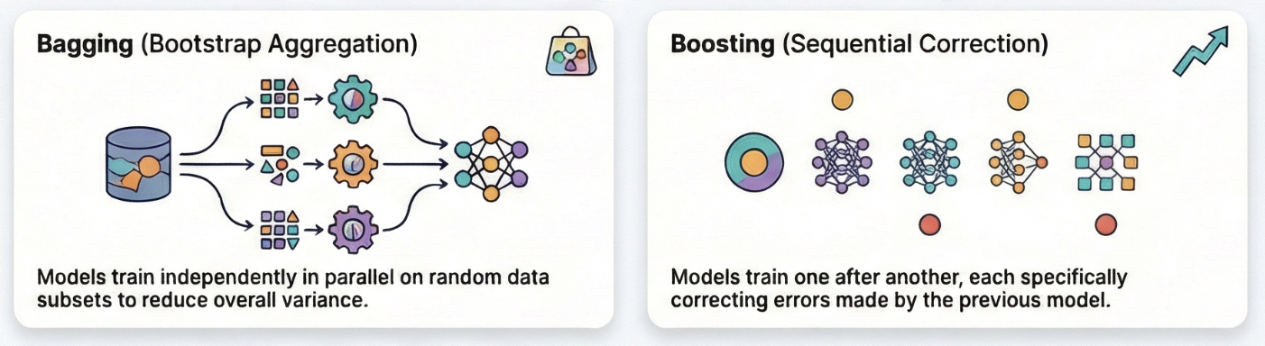
Random Forest builds many trees and averages them.

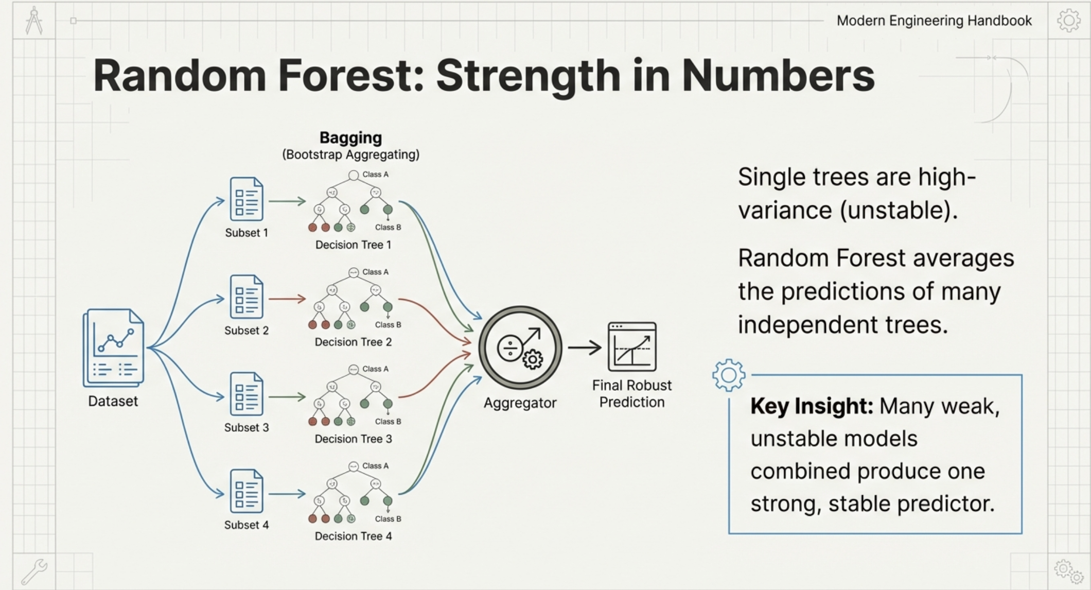
Key idea:

Many weak models combined produce a strong, stable predictor.

Random forests reduce overfitting and improve robustness.

Practical Use Case

Predicting delivery times with many interacting factors:

• traffic
• weather
• route complexity
• warehouse congestion

Random forests handle these nonlinearities effectively.

3.2.1.d. Gradient Boosting and XGBoost (Boosting)

The Industry Workhorse for Regression

Gradient boosting is the most successful regression approach on structured business datasets.

XGBoost is the most widely adopted implementation.

Boosting Intuition: Learning from Mistakes

Boosting builds models sequentially:

• first tree makes predictions
• second tree focuses on errors
• third tree corrects remaining errors
• the ensemble improves step-by-step

This is why boosting is often described as:

An iterative process of error correction.

Why XGBoost Dominates Industry Regression

XGBoost is widely used because it:

• achieves state-of-the-art performance on tabular data
• handles missing values
• captures nonlinear interactions
• scales efficiently
• provides feature importance

Practical Example: Customer Lifetime Value (CLV)

An e-commerce firm predicts Custome Lifetime Value (CLV) as:

CLV = f(PurchaseHistory, Engagement, Discounts, Demographics,…)

CLV drives decisions such as:

• retention investment
• loyalty programs
• premium support allocation

XGBoost is often chosen because:

• accuracy matters financially
• relationships are nonlinear
• interpretability is still possible via feature importance

Hyperparameters That Matter

XGBoost performance depends heavily on tuning:

• tree depth
• learning rate
• number of estimators
• regularization strength

This is why boosting is powerful but requires careful validation.

3.2.1.3 Regression Evaluation Metrics

Regression is evaluated by error magnitude.

Common metrics: We discuss these in WDIS AI-ML Series: Module 2 Lesson 1: Objective function - AI is nothing but an optimization problem

Absolute Error (AE), Mean Absolute Error (MAE), Root Mean Squared Error (RMSE).

Metric Choice is Business Choice

If large errors are catastrophic (pricing, fraud loss), RMSE matters.

If average error is sufficient (forecasting), MAE may be preferred.

‍

3.2.1.4 Regression in Real Organizations

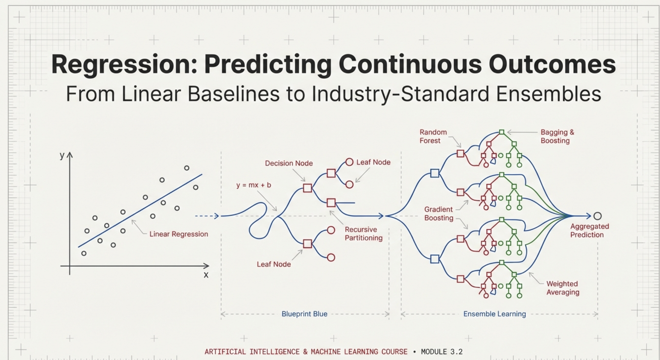
Regression modeling is rarely a one-shot algorithm choice.

Most teams follow a progression:

1. Baseline with linear regression
2. Add regularization for stability
3. Move to trees for nonlinear patterns
4. Deploy XGBoost for high performance
5. Validate with business metrics and monitoring

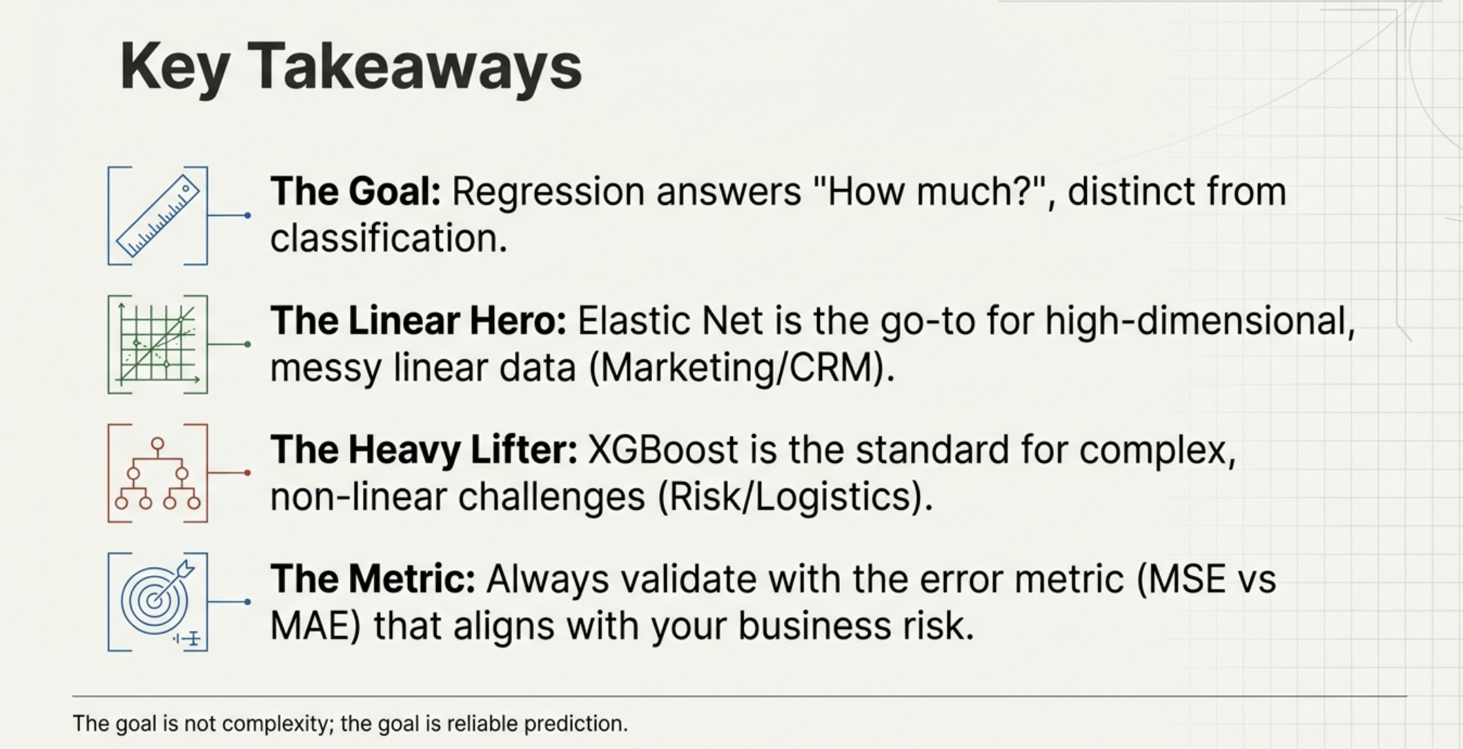
The goal is not complexity.

The goal is reliable numeric prediction that supports decision-making.

Regression Section Summary

Regression models predict continuous numeric outcomes.

They form a hierarchy:

• Linear regression for simplicity and interpretability
• Ridge/Lasso for stability and feature selection
• Tree-based models for nonlinear structure
• Random forests for robustness
• XGBoost for industry-grade performance

Regression is foundational because organizations constantly need to estimate quantities before acting.

Transition: From Regression to Classification

Regression answers: How much?

Classification answers: Which category?

In the next section, we will study classification models, beginning with logistic regression and moving through decision trees, random forests, gradient boosting, support vector machines, and neural networks.